Augmented Reality Plant Disease Detection Using Python, OpenCV, and CNN

prabhu p
Nov 24
8 min read

Augmented Reality Plant Disease Detection

Repository: https://github.com/prabhu31297/Plant-Disease-Detection-using-OpenCV

Introduction

In 2019, during the final phase of my undergraduate degree, I set out to build something that was both technically challenging and directly useful in the real world. Agriculture is still the backbone of India’s economy, yet many farmers lose a significant portion of their harvest because plant diseases are detected too late or misdiagnosed. Diagnosis is still mostly visual—farmers or extension officers walk through fields and visually inspect leaves for spots, discoloration, blights, or fungal growth. This approach does not scale, and it is prone to human error.

My idea was simple: if a smartphone camera can recognize faces and QR codes in real time, why can’t we use a camera to recognize diseased leaves? That question led to Augmented Reality Plant Disease Detection—a system that combines:

Python + OpenCV for real-time image acquisition and preprocessing
Convolutional Neural Networks (CNNs) for disease classification
Augmented Reality overlays for intuitive, real-time feedback

The result is an end-to-end pipeline where a leaf is captured from a live camera, processed, classified, and annotated on-screen with overlaid disease information and recommended actions.

Problem Background: Visual Diagnosis at Scale

Most foliar diseases manifest first on leaves through:

Color shifts (yellowing, browning, chlorosis)
Localized lesions (spots, rings, blisters)
Texture changes (drying, curling, necrosis)
Fungal or bacterial growth (powdery deposits, patches)

An agronomist can often identify the disease from these visual cues, but this depends on experience, lighting, viewing angle, and available time. In a large field, it’s unrealistic to examine every plant—by the time patterns are visible across the field, the disease may already be widespread.

Meanwhile, lab-based detection (microscopy, PCR, etc.) is accurate but:

Time-consuming
Expensive
Not accessible in remote rural areas

Simple “photo upload” apps can help, but they usually:

Work on a single static image
Don’t give live feedback
Don’t visually anchor the result back onto the plant in front of the user

My goal was to bridge this gap using real-time computer vision and deep learning, with the user experience of “point camera → see diagnosis + treatment overlay.”

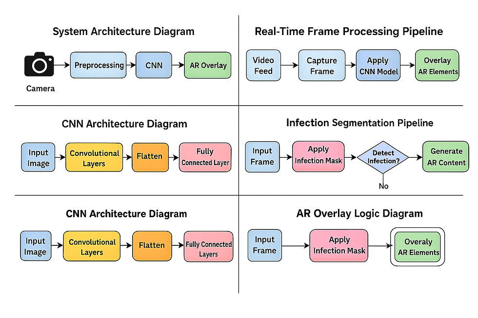
System Architecture Overview

The system architecture has four main modules, wired together into a single pipeline:

Image Acquisition (OpenCV)
Preprocessing & Leaf Segmentation (OpenCV)
Disease Classification (CNN in Keras/TensorFlow)
Augmented Reality Visualization (OpenCV overlays)

At a high level, the flow looks like this:

OpenCV uses VideoCapture() to read frames from a webcam or phone camera.
Each frame is processed to isolate the leaf region from the background.
The segmented leaf patch is normalized and passed to a pre-trained CNN model.
The model outputs disease probabilities → the class with highest score is used.
Using contour geometry, the leaf position is tracked and AR overlays (text and visual cues) are drawn directly on top of the leaf region.

This makes the experience feel like an AR lens: the leaf is “tagged” with its disease name and information as it moves in front of the camera.

Dataset and Preprocessing

Data Sources

The dataset used in this project was assembled from publicly available repositories and research datasets focusing on leaf diseases. It contained:

Multiple disease classes (e.g., Leaf Spot, Blight, Rust, Mosaic Virus, Yellow Leaf Curl, etc.)
A dedicated “healthy” class to teach the model what normal leaf texture looks like
Images with varying lighting, orientation, and background

The goal was not just to perform well on perfectly captured lab images, but to maintain robustness on:

Slightly blurred images
Tilted or rotated leaves
Non-uniform backgrounds

Image Preprocessing

Before training the CNN, each image goes through a standardized preprocessing pipeline:

Resizing:
All images are resized to a fixed dimension (e.g., 128×128 or 224×224) to match the CNN’s input layer.
Color Normalization:
- Convert to RGB if needed
- Scale pixel values to [0, 1] float range for stable training
Data Augmentation:
To improve generalization and simulate real-world variations, I applied augmentations such as:
- Random rotations
- Horizontal flips
- Zoom-in/zoom-out
- Brightness and contrast adjustments
  These were applied on-the-fly during training, so the model sees a different variant of the same image in each epoch.
Background Reduction:
Some preprocessing versions applied leaf-focused masking so the CNN learns leaf texture and lesion patterns instead of memorizing background clutter (soil, lab benches, clothing, etc.).

Together, these preprocessing steps made the model more robust to variations in capture conditions and helped avoid overfitting.

CNN Model Architecture

The disease classification model is built using Keras with TensorFlow backend. Architecturally, it follows the classic Convolution → Nonlinearity → Pooling → Dense pattern.

A typical block in the network looks like:

Conv2D(filters, kernel_size=(3,3), activation='relu')
Optional BatchNormalization()
MaxPooling2D(pool_size=(2,2))

The intuition is:

Early layers learn low-level patterns: edges, color blobs, simple textures.
Deeper layers learn mid–high-level features: lesion shapes, venation patterns, texture irregularities associated with specific diseases.

After several convolutional + pooling blocks, the network flattens the features:

Conv/Pool → Conv/Pool → Conv/Pool → Flatten → Dense → Softmax

Key training details:

Loss function: Categorical cross-entropy
Optimizer: Adam (adaptive learning rate)
Target: Multi-class classification (one disease label per sample)
Output layer: Softmax giving probability distribution across all classes

The model was trained over multiple epochs, with validation monitoring to watch for overfitting. Final accuracy stabilized in the ~92–95% range depending on the train/validation split, which was strong for a student prototype at that time.

Once training was complete, the best-performing model was frozen and exported as an .h5 file. This file is then loaded by the inference script to make live predictions from camera frames.

Real-Time Leaf Detection With OpenCV

The real-time part of the system uses an OpenCV pipeline that prepares each frame for classification.

1. Frame Capture

Using:

cam = cv2.VideoCapture(0)
ret, frame = cam.read()

we continuously read frames from the default camera. Each frame then passes through a series of processing steps.

2. Basic Leaf Segmentation

Real-world frames include tables, walls, clothes, soil, etc. The first goal is to isolate the leaf region:

Color Space Conversion (HSV / HLS)
The frame is converted from BGR to HSV or HLS:

imghls = cv2.cvtColor(frame, cv2.COLOR_BGR2HLS)

Working in HSV/HLS makes it easier to threshold on the “green” hue range corresponding to chlorophyll.
Filtering Near-White Background
In some variants of the code, the algorithm first counts pixels where R, G, B are all above a threshold (e.g., >110). If the percentage of such near-white pixels exceeds ~10%, they are treated as background (e.g., white sheet or flash glare) and downweighted or recolored.
Gaussian Blur + Mean-Shift Filtering
The leaf area is smoothed and homogenized:

blur = cv2.GaussianBlur(img, (3, 3), 1)
img = cv2.pyrMeanShiftFiltering(blur, 20, 30, ...)

Mean-shift filtering reduces noise and small texture variations, making edges and regions more consistent before contour detection.
Edge Detection (Canny)

edges = cv2.Canny(blurred_img, 160, 290)

Canny detects strong gradients, which are then used to find contours.
Contour Detection & Largest Contour Selection

contours, hierarchy = cv2.findContours(...)

max_len = 0
for c in contours:
    if len(c) > max_len:
        max_len = len(c)
        max_id = index

The largest contour (by point count or area) is assumed to be the leaf. Its area (cv2.contourArea) and perimeter (cv2.arcLength) are later used as geometric features.
ROI Cropping Using Bounding Box
A bounding box is computed around the largest contour:

x, y, w, h = cv2.boundingRect(contours[max_id])
roi = img[y:y+h, x:x+w]

This cropped ROI isolates the leaf region and is then resized and normalized before being fed into the CNN.

This pipeline was refined to balance accuracy (proper leaf isolation) and speed (real-time response).

Infection Segmentation and Percentage Calculation

In addition to classification, the project also computes the percentage of leaf area that is infected, using a classical image-processing approach.

Convert ROI to HLS and Focus on Hue Channel

imghls = cv2.cvtColor(roi, cv2.COLOR_BGR2HLS)
hue = imghls[:, :, 0]

Hue encodes color type (e.g., green, yellow, brown). Infection often manifests as color shifts away from healthy green.
Hue Remapping and Masking
The code remaps some hue values (e.g., mapping 0 to 35) and then thresholds:

ret, thresh = cv2.threshold(hue, 28, 255, cv2.THRESH_BINARY_INV)

This produces a binary mask where infected regions (spots, lesions) are separated from healthy tissue.
Masking and Contour Extraction
The binary mask is applied to the original ROI:

mask = cv2.bitwise_and(original_roi, original_roi, mask=thresh)

Then, contours of infected regions are detected:

contours_inf, _ = cv2.findContours(thresh, ...)

Area Calculation
Total infected area is calculated by summing contour areas:

Infarea = sum(cv2.contourArea(c) for c in contours_inf)

The total leaf area Tarea is taken as the area of the main leaf contour or roi.shape[0] * roi.shape[1] as a fallback.
Infection Percentage
Finally:

per = 100 * Infarea / Tarea

This value is displayed as:
Percentage of infection region: XX.XX%

This metric makes the system more informative: it not only tells what disease might be present, but also how severe the infection is.

Augmented Reality Visualization Layer

Rather than just printing the result in the terminal, the project overlays information directly on the camera feed—turning it into a basic AR experience.

Tracking Leaf Position
Using the largest contour, the code computes its centroid (via cv2.moments or bounding box center). This gives (cx, cy) coordinates for placing overlay elements.
Drawing Overlays
Using OpenCV primitives:
- cv2.rectangle() to draw semi-transparent panels near the leaf
- cv2.putText() to display:
  - Disease name
  - Confidence score
  - Infection percentage
  - Short treatment suggestions
For example:

cv2.putText(frame,
            f"Disease: {predicted_label} ({confidence:.2f})",
            (x, y - 10),
            cv2.FONT_HERSHEY_SIMPLEX,
            0.6,
            (0, 255, 0),
            2)

Following the Leaf
Every frame, the contour is recalculated and the bounding box/centroid updated. The overlay is re-drawn at the updated coordinates, making it appear as if the information is attached to the leaf as it moves.
Smoothing (Optional)
To reduce jitter when the leaf moves or segmentation is noisy, a moving average of recent positions can be used to smooth the overlay location.

The result is that a user can move the leaf around in front of the camera and see the disease info visually anchored to the physical object—exactly the kind of interaction that makes AR compelling.

Dataset Logging and Batch Processing Tools

Beyond single-image inference, the repository also includes batch-processing scripts to build labeled datasets and compute geometric features.

The CLI accepts a directory (--input) and walks through all image files.
For each image, the same segmentation pipeline runs, and it computes:
- Leaf perimeter
- Total area
- Infected area
- Infection percentage
The script then asks the user to confirm “infected / not infected”, and appends a row into a CSV file with columns like:

fortnum, imgid, label, feature1 (Tarea), feature2 (Infarea), feature3 (perimeter)

This CSV file can later be used for:

Training classical ML models
Statistical analysis of disease severity
Auditing and improving threshold parameters

It also includes a simple ASCII progress bar in the terminal to visualize batch progress, which is a nice usability touch for long runs.

Challenges Faced During Development

This project touched almost every part of the CV/ML stack, so there were plenty of challenges:

Lighting Variations
Outdoor and indoor lighting drastically changed hue and brightness, sometimes making healthy leaves look diseased or vice versa. I mitigated this with:
- HSV/HLS-based segmentation (more robust to illumination than raw RGB)
- Careful tuning of thresholds across different environments
- Extensive data augmentation in training
Background Clutter
When backgrounds contained other green objects (grass, clothing, plants), segmentation sometimes grabbed the wrong region. To reduce this:
- I prioritized the largest contour
- Used geometric constraints (minimum width/height)
- Applied mean-shift filtering to create cleaner “blobs”
Dataset Imbalance
Some diseases had fewer sample images than others. This was partially mitigated by:
- Aggressive augmentation
- Ensuring the model didn’t overfit to dominant classes during training
AR Overlay Stability
Fast movements produced flickering or misaligned overlays. Smoothing the tracking coordinates over several frames significantly improved perceived stability.

Each of these issues forced me to iterate and refine the pipeline, which in turn strengthened my understanding of both computer vision and deployment constraints.

Real-World Applications

Even though this started as an academic project, it hints at several real-world use cases:

Mobile assistant for farmers:
A smartphone app that allows farmers to scan leaves and get immediate feedback.
Drone- or rover-based monitoring:
Integrating the model into a drone or ground robot to rapidly scan sections of a field.
Insurance and verification:
Insurance providers could use standardized visual evidence to verify disease-related claims.
Research and teaching tools:
Agricultural universities and labs could use such tools to teach disease identification and to collect labeled datasets efficiently.

The combination of computer vision, deep learning, and AR turns disease detection into an interactive, educational experience instead of a black-box prediction.

Conclusion

My Augmented Reality Plant Disease Detection project was more than an academic exercise—it was an exploration of how artificial intelligence can meaningfully impact agriculture. By combining Python, OpenCV, and CNNs, I created a system that detects plant diseases in real-time and communicates the results through an intuitive AR interface. The project gave me deep exposure to computer vision, machine learning, and human-centered design, and it remains one of the projects I’m most proud of from my undergraduate journey.

You can view the complete source code on GitHub here:

https://github.com/prabhu31297/Plant-Disease-Detection-using-OpenCV